Point Matching

Point matching is the task of finding correspondences between two arbitrary sets of points. Usually one point set is designated the model set, and the other the data set. Associated with any given set of correspondences is a geometric transformation, which represents the position, or pose, of the model set within the data set. When this transformation is applied to the model, the position of the model points resembles that of the data points.

Heuristically Seeded Local Search

The Denton/Beveridge point matching algorithm is a heuristically guided local search algorithm for point matching that performs well even in the presence of spurious points in the model and data sets. The algorithm begins with a small set of paired points, and then seeks to improve upon that match. Each possible single addition, removal, and swap is considered. If one or more possible improvements are found, the best improvement is applied to the existing match set and the process begins again. When no further improvement is found, the search terminates. The quality of each match set is judged based on the number of model points matched, the error between the transformed model and the data, and a penalty for sets of matches that represent an unlikely geometric transformation.

Beginning a search with a random set of points is unlikely to produce a good result, so the Denton/Beveridge point matching algorithms uses a simple heuristic to construct initial matches to begin the search. This heuristic is based on the observation that groups of model points that are close to each other should map to groups of data points that are also close together. A list of all possible mappings between neighboring model points and neighboring data points is constructed. This list then provides the starting points for a number of different rounds of local search, as previously described.

When there are few spurious points in the model and data set, the heuristic algorithm frequently identifies starting points that will quickly lead the local search algorithm to a correct solution. When there are more spurious points, a larger portion of the list of starting points must be search before a good solution is found. Fortunately, the local search algorithm is very fast and it can be run many times is a short period of time. As more trials are run, the chance that they have all failed to find a good solution drops towards zero.

Although this algorithm is very fast, it frequently does not result in a good match. To compensate, the algorithm can be run many times. As the algorithm is run repeatedly, the chance that every attempt will fail drops zero. With enough iterations, it becomes possible to be confident that the best solution has been found. In practice, the combination of the heuristic start algorithm and local search often finds solutions to point matching problems that RANSAC can not, and does so faster than other traditional search techniques.

An Example

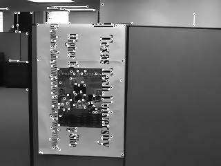
An example will be helpful. Start with two images, such as those shown below. The image on the left will provide the model, the one on the right will be the data.

First, identify all the corner points in these images, using some automated feature detector such as the Harris corner extractor. This results in model and data point sets.

These points, and only the information about the point location, is feed into the point matching software. The program "sees" only something that looks like the images below.

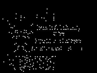
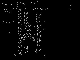
The algorithm first identifies groups of neighboring points in each set, and then constructs partial match sets by pairing the groups. For example, consider the four points on the T and E in the word Texas. These corners are visible in both sets. These four points are paired in every possible combination and each grouping feeds one trial of local search. One of the groupings is correct, and leads the search algorithm to a series of additional pairs that completes the match.

At the end the point matching software reports a set of correspondences and an optimal pose like that shown below.

( 18, 70) ( 20, 23) ( 21, 20) ( 22, 43) ( 23,109) ( 24,123) ( 25,151) ( 26, 87) ( 29,177) ( 30,153)
( 31, 48) ( 32, 56) ( 33, 93) ( 34,137) ( 36, 67) ( 40, 54) ( 41,104) ( 42, 77) ( 43,157) ( 44,180)
( 45, 50) ( 46, 62) ( 47, 66) ( 48, 83) ( 49, 95) ( 51,114) ( 52,125) ( 53,136) ( 54,146) ( 55,152)
( 56,159) ( 57,161) ( 59,171) ( 60, 42) ( 61,  0) ( 65,178) ( 66, 18) ( 71,  7) ( 76, 28) ( 77,120)
( 78,130) ( 81,132) ( 82,139) ( 87,118) ( 88,141) ( 99, 37) (100,128) (101, 76) (102, 84) (104, 46)
(105, 55) (107,170) (108,179) (109, 58) (110,103) (111,116) (114,164) (115,168) (116,173) (117, 65)
(119, 38) (120,169) (123, 61) (124, 80) (125, 96) (126,117) (127,131) (128,142) (131,181) (132, 36)
(133, 63) (134, 75) (135, 86) (136, 51) (137,167) (141,  6) (146, 27) (147, 59) (148, 64) (149,121)
(150,156) (151, 39) (153, 82) (154, 26) (155, 53) (156, 94) (157,107) (159,182) (163,158) (164,122)
(165, 32) (166, 74) (167, 92) (168,102) (169,115) (170,183) (172, 52) (173, 57) (174, 97) (175,108)
(176,  3) (177,155) (180, 12) (181, 14) (187, 21) (199, 11) (216, 73) (222, 10) (223, 34) (228, 22)
(232, 71) (234, 33) (236,  9) (238, 29) (247,  4) (253, 69) 
Pairs: 116 Fitness: 170.8152
a: 0.015431 b: -1.110821 c: 261.447825 
d: 1.201859 e: 0.037866 f: -91.858356 
g: 0.000094 h: 0.000563

The optimal pose can then be used to transform the model set to look like the data set. If we transform the first image to look like the second, and then overlay that with the original second image, we end up with the following.

Papers

Details of our technique can be found in the following papers. Citation information for this papers is available in a BibTex file.

Software

The source code for a highly optimized version of this technique is available. Sample data files are included.

Source Code